TEA RATING: ☕
If you are struggling to query your date in an excel sheet, you can use index(match()) formula to lookup. Unlike vlookup or hlookup, index(match()) is more flexible and more roboust.
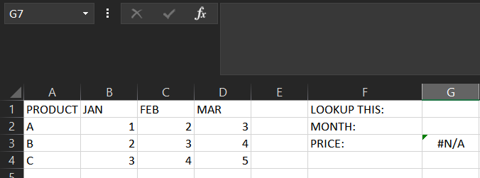
Let’s start with this situation, you have a group of product prices in a list from different months.

As you can gues we will enter the product name we want to have a look at G1 cell, month to G2 cell and get the results for different months at G3.
So the formula works like this;
INDEX(<RANGE FOR YOUR RETURN DATA>;MATCH(<CELL TO BE LOOKED UP>;<WHERE TO SEARCH THAT CELL>;<“0” FOR EXACT MATCH>);<COLUMN THAT YOU WANT TO RETURN FROM THE RANGE>)
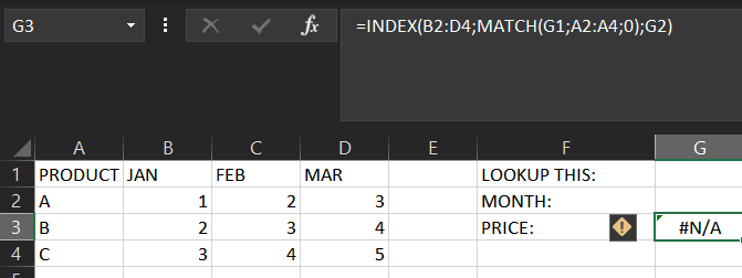
For this case will be like here;
=INDEX(B2:D4;MATCH(G1;A2:A4;0);G2)

So if you try with product “A”, in month “2” which is feb, (here user actually entering a column); then you will get 2 as a result;

Please also be aware that you may not enter any value to G2 which is month and you will get all the date responding to product “A” like below;

So it is also possible to return multiple date with this great tool.